Reinforcement Learning Basics: Q Learning

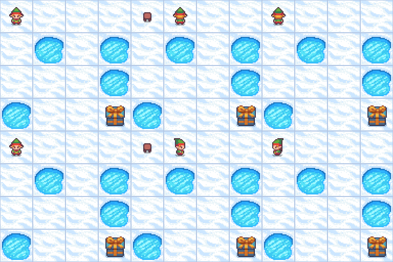
Imagine teaching a robot to cross a room without bumping into furniture. You could give it a set of instructions, but what if the room changes every time? That’s where Reinforcement Learning (RL) comes in—specifically, Q-Learning, one of the most fundamental and powerful algorithms in RL.

In this blog, we’ll explore what Q-learning is, how it works, where it's used, and how you can implement it from scratch for the Frozen Lake Environment of Gym.

1. What is Q-Learning?

Q-Learning is a model-free, value-based reinforcement learning algorithm. It helps an agent learn how to act optimally in a given environment by learning the value (or quality) of actions taken in specific states.

The goal is to learn the Q-function:

$$Q(s,a)=\text{Expected future reward of taking action }a\text{ in state }s$$

Over time, the agent updates its Q-values by interacting with the environment, receiving rewards, and adjusting its future behavior accordingly.

2. Bellman Optimality Equation

Bellman optimality principle states that the optimal value of a state can be computed based on the immediate reward and the optimal value of the next state.

i) Value for Action (Q-Value)

where:

Qπ(s,a)- It is the Q-Value for the current state(s) taking action(a).

P(s′∣s,a)- It is the probability of transition from state(s) to next state(s') if action(a) is taken.

$R(s,a)-$It is the reward for taking action(a) at state(s).

γ- It is the discount factor which implies the importance of future rewards.

$\pi (a|s)-$The probability of taking action(a) in state(s). 

ii) Value for State (V)

where:

V*(s)-Maximum expected return from state(s).

• Q-Value basically states what is the max reward by taking this particular action.
• Whereas the state value tells us what is the action that can be taken in this state to get max reward.

3. How to proceed with Q-Learning?

To understand Q-Learning intuitively, let’s walk through an example using a 5×5 grid world. The goal is for an agent (robot) to navigate from a start position to a goal position, while avoiding traps and maximizing cumulative reward. The environment is deterministic: if the agent takes an action, it moves in that direction unless it hits a wall.

The agent starts with a Q-table initialized to zeros:

$$Q(s,a)=0\text{for all }s\in \text{states},a\in \text{actions}$$

As it explores the environment using ε-greedy policy, the agent updates its Q-values using:

$$Q(s,a)\leftarrow P(s|s\text{'},\; a)*\; [r+\mathrm{max <span\; class="vlist-s"></span>}\underset{{\mathrm{<br>}}^{}}{\mathrm{<span\; class="mspace"></span><span\; class="mop\; op-limits"></span>}}Q(s^{\mathrm{\prime }},a^{\mathrm{\prime }})]$$

The agent keeps playing the episodes and explores the states and keeps updating the q_value. If you are familiar with dynamic programming, then it is similar to that principle.

Finally, after some iterations, the agent learns to take optimal values.

4. Exploration vs Exploitation

Q-Learning uses an ε-greedy strategy:

• With probability $\varepsilon$, the agent explores (random action).

• With probability $1 - \varepsilon$, it exploits (chooses best known action).

This ensures the agent doesn’t get stuck in a suboptimal strategy early on.

5. The Frozen Lake Environment

The FrozenLake environment is a classic benchmark from OpenAI Gym used to test reinforcement learning algorithms in a discrete grid-world setting. It represents a frozen lake where an agent must learn to navigate from a start point to a goal without falling into holes. The environment is structured as a grid of tiles that can be:

• S: Start

• F: Frozen (safe)

• H: Hole (game over if entered)

• G: Goal

The challenge comes from the slippery surface, which introduces stochasticity—the agent may slip and end up in a different tile than intended. This forces the agent to learn a policy that balances risk and reward, making it ideal for studying exploration, stochastic transitions, and reward sparsity in reinforcement learning.

6. Implementation

The main highlights of the code are:

1. Q-table: Initialized to zeros.
2. Transition table: Tracks how often a state transitions to another.
3. Reward dictionary: Maps (state, action, next_state) to reward values.
4. play_n_random_episodes(n): Random exploration to populate experience.
5. value_iteration(): Updates Q-values based on observed transitions.
   
6. play_episode(): Runs one episode using the current Q-table greedily.
7. Stopping condition: Training stops when the agent achieves an average reward above 0.8 across test episodes.

The code can be found in this repository. I have tried my best to make it as clear as possible, so that the theory can be closely followed.

Code: Q-Learning

With enough exploration, the agent eventually learns a reliable policy to reach the goal. Training may converge in as few as 10 episodes or take up to 200, depending on how efficiently it explores and generalizes from the observed transitions.

7. Conclusion

In this article we have gone through the theory of Q-Learning Method and tried to understand how to implement it from scratch. Next, we will look at how neural networks can help us in estimating the Q-Values. Thank You and Stay Tuned.

FUTURE BEYOND OUR STAR!