Reinforcement Learning Basics: Deep Q Learning Networks (DQN)

 

In traditional Q-Learning, we store a Q-table to estimate the expected return for every state-action pair. But what happens when the state space is huge—or even continuous? That’s where Deep Q-Networks (DQN) come into play.

In this blog, we’ll explore what DQN is, how it works, and test it out on the famous Atari environment of Breakout. It would be better if you can familiarize yourself with Q-Learning that has been explained in previous blog, before proceeding further.

1. What is Deep Q-Learning?

DQN merges Reinforcement Learning with the power of Deep Learning. Instead of a lookup table, it uses a neural network to approximate the Q-function. This breakthrough led to monumental achievements like DeepMind’s DQN agent learning to play Atari games directly from raw pixel input—outperforming humans in many of them.

This approach can handle:

• High-dimensional state spaces (like raw images)

• Generalization across unseen states

• Continuous learning in dynamic environments

2. The Bellmann Update and Target Network

DQN follows the same method of calculating the Q-Values as in Q-Learning explored before. One key difference is that this Q-Value is obtained using the target network and is used as a target value for the main network to calculate the loss as follows:

where:

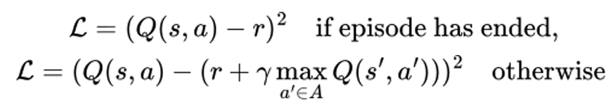
Q(s,a) - It is the current q value predicted by the network for action a.

Q(s',a') - Is the target q value predicted by target network for next state(s') and action(a').

γ - It is the discount value which emphasizes the impact of future reward.

The target net is used to make the training more stable. This network is then synchronized with our main network periodically for every n steps.

3. Replay Buffer 

One of the fundamental assumptions behind Stochastic Gradient Descent (SGD) is that training samples are independent and identically distributed (i.i.d). This means that each training example should be drawn randomly and independently from the data distribution.

However, in reinforcement learning, the data collected from the environment—specifically frames or transitions—are sequentially correlated. This violates the i.i.d assumption and can lead to unstable learning or convergence to suboptimal policies.

To mitigate this, we use a technique called Experience Replay.

• As the agent interacts with the environment, we store transitions in the form of:

  $$(s,a,r,s^{\mathrm{\prime }},\text{done})$$

  in a large buffer (deque).

• Rather than training on the most recent transition, we randomly sample batches from this buffer after enough experiences are collected.

This randomization breaks the correlation between consecutive transitions, improves sample efficiency, and makes the training process more stable and generalizable—which is critical for learning from high-dimensional inputs like video frames in Atari games.

4. The Markov Property

A typical Markov Process

Reinforcement Learning (RL) methods are typically built on the framework of a Markov Decision Process (MDP). An MDP assumes that the environment satisfies the Markov Property—that is, the current observation contains all the information necessary to make an optimal decision.

However, this assumption often breaks down in real-world scenarios or complex games like Atari Breakout. In Breakout, for example, a single frame may not convey crucial information such as the velocity or direction of the ball. This makes the environment a Partially Observable Markov Decision Process (POMDP)—where observations are incomplete representations of the true state.

To handle this, we use a common trick in deep RL: frame stacking.

Instead of using one image as the agent’s observation, we stack the last $k$ frames (typically $k=4$) together. This provides temporal context and allows the agent to infer motion, such as how fast and in which direction the ball is moving. In doing so, we effectively convert the POMDP into an approximate MDP, enabling the agent to make informed decisions based on short-term dynamics.

Frame stacking is simple but powerful—it’s one of the key innovations that made deep reinforcement learning work on vision-based tasks like Atari games.

5. The Breakout Environment

The Breakout environment from the Atari 2600 suite is a classic benchmark used in reinforcement learning research. The player (or agent) controls a paddle at the bottom of the screen, aiming to bounce a ball upward to break bricks arranged at the top. 

The game challenges the agent to learn timing, positioning, and ball dynamics to maximize score while avoiding the ball falling past the paddle. Breakout is especially useful in deep RL because it involves sparse rewards, temporal dependencies, and requires visual perception from raw pixel inputs—making it an ideal testbed for algorithms like DQN.

6. Implementation

The main highlights of the code are:

1. CNN-based Q-Network
   
   
   
   
   
2. Experience Replay: The Buffer holds up to 1 million transitions and samples the given batch size.

   

   
   
3. Reward Truncation: The episode ends early if info['lives'] < 5, forcing the agent to prioritize life retention.
4. Training Flow: 

• Start playing randomly until the buffer fills with 50,000 transitions.
• Once enough data is gathered, begin training the Q-network every step.
• Synchronize target network every 1000 frames.
• Decay epsilon over time to shift from exploration to exploitation.
• Track reward, epsilon, and loss via TensorBoard.

The code can be found in this repository. I have tried my best to make it as clear as possible, so that the

theory can be closely followed.

Code: DQN

Despite the textbook structure, the agent failed to consistently improve. The best score achieved was 5, which is better than random—but far from solving the environment.

7. Conclusion

Training DQN on Breakout from scratch is notoriously difficult. The original DeepMind paper took 8 GPUs, 200 million frames, and sophisticated tweaks. While my setup followed the core ideas faithfully, a few practical limitations (single-GPU GTX 1650, short training window, unoptimized hyperparameters) likely held back performance.

Still, this project offered a realistic glimpse into the complexity of deep RL in high-dimensional environments.Thank You and Stay Tuned.

FUTURE BEYOND OUR STAR!